VLOOKUP and HLOOKUP are probably the best-known formulas for getting data from another table. It is relatively simple to use as long as you are looking to just retrieve one data point using one criteria and the table (number of columns) never changes. However, SUMIFS are quickly becoming more used as users are looking at increasingly more detailed data sets and need to summarize the data across several dimensions.
Occasionally you can use a combination of LOOKUP and pivot tables to get to a summary result, but it quickly becomes cumbersome and difficult to update. SUMIFS can do much of what VLOOKUP can do but with even more functionality. SUMIFS doesn’t care about the column order or if new columns are added in between the lookup and return columns. SUMIFS returns the sum of all matching values and zero if there are no matching values. And finally, SUMIFS can look up or sum up values based on multiple criteria rather than just one
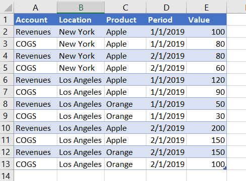
Imagine a scenario where you are looking at a data sheet with revenues and cost of goods by location, product and period and want to be able to get the data in a summary format:

Rather than creating a Pivot Table to then copy and paste it or link to the table, you can use a simple SUMIFS function to get the sum of the data. SUMIFS are written in the following order inside the SUMIFS brackets of which the first three terms are required:
- The cell reference with the values you want to sum up.
- The cell reference containing your criteria for eventual evaluation.
- The lookup value (your criteria).
- Optional: Second criteria column.
- Optional: Second lookup value.
- Etc.
For example, say you want Revenues in Los Angeles for January 2019. You would use the SUMIFS formula as follows:
=SUMIFS(E2:E13,B2:B13,”Los Angeles”,A2:A13,”Revenues”,D2:D13,”1/1/2019″)
The first part (E2:E13) contains the values you want to sum up. The second part (B2:B13) contains the column you want to lookup for the first criteria (“Los Angeles”). After that, it is optional how many criteria you want to add. In this example, we are also looking for “Revenues” in column A2:A13 and “1/1/209” in column D2:D13. If you do this, you should get a value of 170.
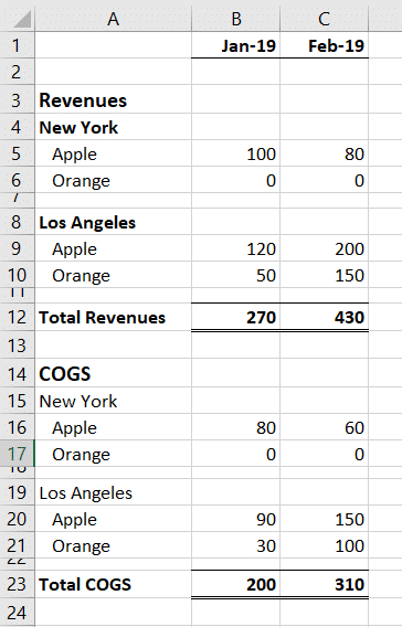
You can take this further and use SUMIFS functionality to summarize the entire data set into a basic P&L template displaying Revenues and COGS by location and product that looks like this:

The formula in cell B5 looks like this:

=SUMIFS(‘Data Set 1′!$E:$E,’Data Set 1′!$A:$A,’Summary 1′!$A$3,’Data Set 1′!$B:$B,’Summary 1′!$A$4,’Data Set 1′!$C:$C,’Summary 1′!$A5,’Data Set 1′!$D:$D,’Summary 1’!B$1)
‘Data Set 1’ is the Excel tab where the data lives. As you can see, it sums up column E based on looking up four criteria: The account, the location, the product and the period. When you reference cells as the lookup criteria, the only thing you need to be careful of is ensuring there are no typos or extra spaces. You also need to make sure that each column has the same number of rows in the formula (i.e., if you select row 2 to 13 for one criterion, you have to make sure ALL criteria reference row 2 to 13). Now, you can lock in the cells and copy the formulas across each column and row while ensuring the formulas use the correct lookup criteria to get to the summary P&L displayed above.
As you can see, it is a quick tool to use to sum up data. You can obviously use this formula to look up both vertically and horizontally depending on how the underlying data is displayed. As you get more comfortable with this functionality, you can edit the lookup criteria to be more sophisticated to include conditions such as greater or equal to (>=), unequal (<>), wildcards (*) etc.
Learn More. Become a Subscriber.

